01 Examples#
[1]:
%reload_ext autoreload
%autoreload 2

import os
from pathlib import Path
import numpy as np
from scipy.integrate import simpson, trapezoid
from pytrunc.phase import calc_moments, henyey_greenstein, calc_hg_moments
from pytrunc.truncation import delta_m_phase_approx, gt_phase_approx
from pytrunc.utils import integrate_lobatto, quadrature_lobatto

import matplotlib.pyplot as plt
from matplotlib.ticker import MaxNLocator
import xarray as xr
from pytrunc.constant import DIR_ROOT
Compute all truncated phase matrix unique terms#
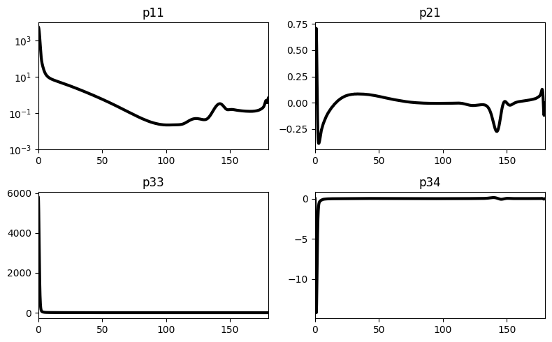
Water cloud#
spherical particle
Get realistic water cloud phase function from mie calculation#
[2]:
# in the paper (Iwabuchi et al. 2009) water cloud at wl = 500 nm and reff = 8 um

# wc available in smartg auxdata: https://github.com/hygeos/smartg
# Follow smartg README to download auxdata,
# then create environemnt variable 'SMARTG_DIR_AUXDATA' where auxdata have been downloaded
# wc_path = Path(os.environ['SMARTG_DIR_AUXDATA']) / Path('clouds/wc_sol.nc')
# ds = xr.open_dataset(wc_path)
# pha_exact = ds['phase'].interp(reff=8, wav=500, method='linear').values[0, :]

# wc at the correct wavelength and effective radius avaible in pytrunc/data
ds = xr.open_dataset(DIR_ROOT / 'pytrunc' / 'data' / 'wc_wl500_reff8.nc')

theta = ds['theta'].values
pha_ex = ds["phase"].values

method = 'lobatto'
# method = 'trapezoid'
# method = 'simpson' # use pair number for theta

INTEGRATORS = {
    "simpson": simpson,
    "trapezoid": trapezoid,
    "lobatto": integrate_lobatto
    }
integrate_m = INTEGRATORS[method]

# theta = np.linspace(0., 180., 18001)
# pha_ex = np.interp(theta, ds.theta.values, pha_ex)

# theta, _ = quadrature_lobatto(0., 180., 7201)
# pha_ex = np.interp(theta, ds.theta.values, pha_ex)

mu = np.cos(np.deg2rad(theta))
idmu = np.argsort(mu)


# renormalize depending on the chosen integration method
if method == 'lobatto':
    sin_th = np.sin(np.deg2rad(theta))
    pha_ex = (2. * pha_ex) / integrate_m(pha_ex[0,:]*sin_th, np.deg2rad(theta))
else:
    pha_ex = (2. * pha_ex) / integrate_m(pha_ex[0,idmu], mu[idmu])


fig, axs = plt.subplots(2, 2, figsize=(8,5))
axs = axs.ravel()
axs[0].plot(theta, pha_ex[0,:], 'k-', lw=3, label='p11 exact')
axs[0].set_yscale('log')
axs[0].set_ylim(1e-3, 1e4)
axs[0].set_xlim(0, 180)
axs[0].set_title('p11')
axs[1].plot(theta, pha_ex[1,:], 'k-', lw=3, label='p21 exact')
axs[1].set_xlim(0, 180)
axs[1].set_title('p21')
axs[2].plot(theta, pha_ex[2,:], 'k-', lw=3, label='p33 exact')
axs[2].set_xlim(0, 180)
axs[2].set_title('p33')
axs[3].plot(theta, pha_ex[3,:], 'k-', lw=3, label='p34 exact')
axs[3].set_xlim(0, 180)
axs[3].set_title('p34')
plt.tight_layout()
plt.show()
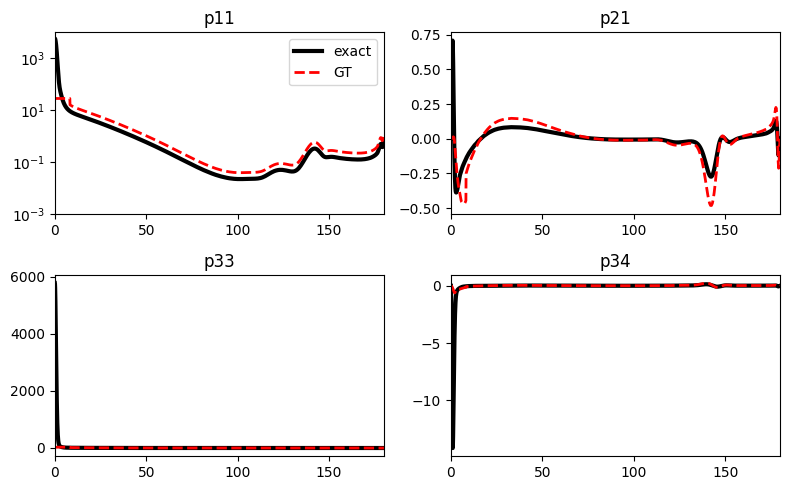
Truncated phase matrix using the GT method#
Iwabuchi 2009
[3]:
# Get the f value equal to chi_20
m_max = 20
chi = calc_moments(pha_ex[0,:], theta, m_max=m_max, normalize=True)
f = chi[m_max]
print('f=', f)

ds_gt = gt_phase_approx(pha_ex[0,:], theta, f, method=method,
                                        phase_moments_1=chi[1], th_tol=20.)

# Eq.5 in Waquet and Herman, 2019
pha_tr = np.zeros_like(pha_ex)
pha_tr[0,:] = ds_gt['phase_tr'].values
beta = (pha_tr[0,:] / pha_ex[0,:])
for i in range(1, pha_ex.shape[0]):
    pha_tr[i,:] = pha_ex[i,:] * beta

fig, axs = plt.subplots(2, 2, figsize=(8,5))
axs = axs.ravel()
axs[0].plot(theta, pha_ex[0,:], 'k-', lw=3, label='exact')
axs[0].plot(theta, pha_tr[0,:], 'r--', lw=2, label='GT')
axs[0].set_yscale('log')
axs[0].legend()
axs[0].set_ylim(1e-3, 1e4)
axs[0].set_xlim(0, 180)
axs[0].set_title('p11')
axs[1].plot(theta, pha_ex[1,:], 'k-', lw=3)
axs[1].plot(theta, pha_tr[1,:], 'r--', lw=2)
axs[1].set_xlim(0, 180)
axs[1].set_title('p21')
axs[2].plot(theta, pha_ex[2,:], 'k-', lw=3)
axs[2].plot(theta, pha_tr[2,:], 'r--', lw=2)
# axs[2].set_yscale('log')
# axs[2].set_ylim(-1., 1)
axs[2].set_xlim(0, 180)
axs[2].set_title('p33')
axs[3].plot(theta, pha_ex[3,:], 'k-', lw=3)
axs[3].plot(theta, pha_tr[3,:], 'r--', lw=2)
axs[3].set_xlim(0, 180)
axs[3].set_title('p34')
plt.tight_layout()
#plt.savefig('truncated_phase_gt.png', dpi=300)
f= 0.43294807007378455
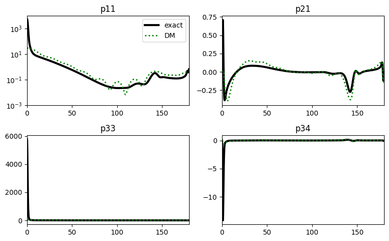
Truncated phase matrix using the delta-M method#
Wiscombe et al. 1997
[4]:
# Get the f value equal to chi_20
m_max = 20
ds_dm = delta_m_phase_approx(pha_ex[0,:], theta, m_max, method=method)
f = chi[m_max]
print('f=', f)

# Eq.5 in Waquet and Herman, 2019
pha_tr = np.zeros_like(pha_ex)
pha_tr[0,:] = ds_dm['phase_tr'].values
beta = (pha_tr[0,:] / pha_ex[0,:])
for i in range(1, pha_ex.shape[0]):
    pha_tr[i,:] = pha_ex[i,:] * beta

fig, axs = plt.subplots(2, 2, figsize=(8,5))
axs = axs.ravel()
axs[0].plot(theta, pha_ex[0,:], 'k-', lw=3, label='exact')
axs[0].plot(theta, pha_tr[0,:], 'g:', lw=2, label='DM')
axs[0].set_yscale('log')
axs[0].legend()
axs[0].set_ylim(1e-3, 1e4)
axs[0].set_xlim(0, 180)
axs[0].set_title('p11')
axs[1].plot(theta, pha_ex[1,:], 'k-', lw=3)
axs[1].plot(theta, pha_tr[1,:], 'g:', lw=2)
axs[1].set_xlim(0, 180)
axs[1].set_title('p21')
axs[2].plot(theta, pha_ex[2,:], 'k-', lw=3)
axs[2].plot(theta, pha_tr[2,:], 'g:', lw=2)
axs[2].set_xlim(0, 180)
axs[2].set_title('p33')
# axs[2].set_yscale('log')
# axs[2].set_ylim(-1., 1)
axs[2].set_xlim(0, 180)
axs[2].set_title('p33')
axs[3].plot(theta, pha_ex[3,:], 'k-', lw=3)
axs[3].plot(theta, pha_tr[3,:], 'g:', lw=2)
axs[3].set_xlim(0, 180)
axs[3].set_title('p34')
plt.tight_layout()
#plt.savefig('truncated_phase_dm.png', dpi=300)
f= 0.43294807007378455
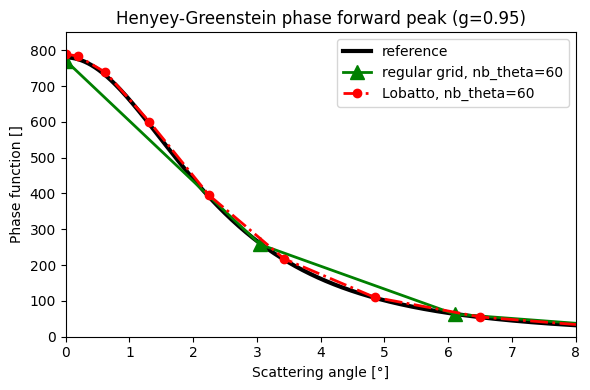
Use Lobatto for an accurate phase function with lesser angle points#
Interesting for particles with a high forward or backward peak.
A phase function with lesser angle points allows to save memory and computional time in some radiative transfer codes
Example with the Henyey-Greentein phase function#
[5]:
nb_th = 60
theta_lob, _ = quadrature_lobatto(0., 180., nb_th)
theta_reg = np.linspace(0, 180., nb_th)
hg_phase_lob = henyey_greenstein(theta_lob, g=0.95, normalize=2)
hg_phase_reg = henyey_greenstein(theta_reg, g=0.95, normalize=2)

hg_phase_ref = henyey_greenstein(np.linspace(0, 180., 18001), g=0.95, normalize=2)

plt.figure(figsize=(6,4))
plt.plot(np.linspace(0, 180., 18001), hg_phase_ref, 'k-', lw=3, label='reference')
plt.plot(theta_reg, hg_phase_reg, 'g-^', lw=2, ms=10, label=f'regular grid, nb_theta={nb_th}')
plt.plot(theta_lob, hg_phase_lob, 'r-.o', lw=2, ms=6, label=f'Lobatto, nb_theta={nb_th}')
plt.ylim(0, 850)
plt.xlim(0, 8)
plt.title('Henyey-Greenstein phase forward peak (g=0.95)')
plt.xlabel('Scattering angle [°]')
plt.ylabel('Phase function []')
plt.legend()
plt.tight_layout()
#plt.savefig('hg_phase_forward_peak.png', dpi=200)
Example with moment calculations#
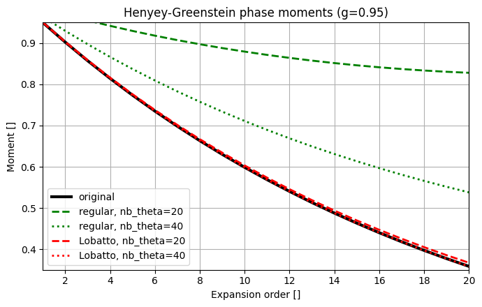
[6]:
m_max = 20
chi_exact = calc_hg_moments(0.95, m_max)
nth = np.array([20, 40])
expansion_order = np.arange(0, m_max + 1)
marks = ['--', ':']


plt.figure(figsize=(7,4.5))
plt.plot(expansion_order, chi_exact, 'k-', lw=3, label='original')
for ith in range (len(nth)):
    theta_reg = np.linspace(0, 180., nth[ith])
    hg_reg = henyey_greenstein(theta_reg, g=0.95, normalize=2)
    chi_reg = calc_moments(hg_reg, theta_reg, m_max, method='trapezoid', normalize=True)
    plt.plot(expansion_order, chi_reg, f'g{marks[ith]}', lw=2, label=f'regular, nb_theta={nth[ith]}')

for ith in range (len(nth)):
    theta_lob, _ = quadrature_lobatto(0., 180., nth[ith])
    hg_lob = henyey_greenstein(theta_lob, g=0.95, normalize=2)
    chi_lob = calc_moments(hg_lob, theta_lob, m_max, method='lobatto', normalize=True)
    plt.plot(expansion_order, chi_lob, f'r{marks[ith]}', lw=2, label=f'Lobatto, nb_theta={nth[ith]}')

plt.title('Henyey-Greenstein phase moments (g=0.95)')
plt.xlabel('Expansion order []')
plt.ylabel('Moment []')
plt.ylim(0.35, 0.95)
plt.xlim(1, 20)
plt.gca().xaxis.set_major_locator(MaxNLocator(integer=True))
plt.grid()
plt.legend()
plt.tight_layout()
#plt.savefig('hg_phase_moments_convergence.png', dpi=200)