Gaseous absorption correction

1 Overview

The correction for the gaseous absorption of various gases is applied before Rayleigh correction, thus the coupling between absorption and scattering is neglected. The gaseous-corrected reflectance is obtained from the TOA reflectance as:

\[\rho_{\text{gc}} = \frac{\rho_{\text{TOA}}}{t_g}\]

where \(\rho_{\text{TOA}}\) is the top-of-atmosphere reflectance and \(t_g\) is the gaseous absorption transmittance along the downward + upward (solar and sensor view) path.

The eotools.gaseous_correction module provides several classes implementing a generic correction for gaseous absorption:

Gas	Gas_correction_CKDMIP	Gas_correction_O3	Gas_correction_NO2
References	(Hogan and Matricardi 2022; Anderson et al. 1986)	NASA O3	NASA NO2
CH₄	✓
CO₂	✓
H₂O	✓
N₂	✓
N₂O	✓
O₂	✓
O₃	✓	✓
NO₂			✓

• Gas_correction_O3 & Gas_correction_NO2: Legacy correction modules using absorption cross-section data integrated with the sensor SRF.
• Gas_correction_CKDMIP: Modern correction using the CKDMIP high-resolution line-by-line transmission model, supporting multiple absorbing gases simultaneously.

Gas_correction is a proxy to the above classes. By default, it uses Gas_correction_O3 and Gas_correction_NO2, but Gas_correction_O3 can be replaced by Gas_correction_CKDMIP via an option.

1.1 Gas_correction_O3

The Gas_correction_O3 class corrects for ozone (O₃) absorption using cross-section data from NASA Ocean Color (Anderson et al.). The absorption coefficient \(K_{\text{O}_3}\) is computed per band by integrating the cross-section data with the sensor SRF, or by interpolation at central wavelengths when no SRF is available.

The correction follows the Beer-Lambert law:

\[T_{\text{O}_3} = \exp(-K_{\text{O}_3} \cdot U_{\text{O}_3} \cdot M)\]

where \(U_{\text{O}_3}\) is the total column ozone in Dobson Units and \(M\) is the air mass factor. The TOA reflectance is then divided by the transmittance: \(\rho_{\text{gc}} = \rho_{\text{TOA}} / T_{\text{O}_3}\).

Inputs required: Total column ozone (Dobson Units), air mass.

2 Gas_correction_NO2

The Gas_correction_NO2 class corrects for nitrogen dioxide (NO₂) absorption using cross-section data from NASA Ocean Color (Bogumil et al. 2003). The absorption coefficient \(K_{\text{NO}_2}\) is computed per band by integrating with the sensor SRF or by interpolation at central wavelengths.

NO₂ column amounts are derived from climatology data (HDF files) combined with a tropospheric NO₂ factor at 200 m resolution. The correction follows the same Beer-Lambert transmission model as O₃.

Inputs required: Latitude, longitude, acquisition date (for climatology lookup), air mass.

3 CKDMIP

The Gas_correction_CKDMIP class provides modern gaseous correction using the CKDMIP high-resolution line-by-line transmission model.

3.1 High spectral resolution line-by-line dataset

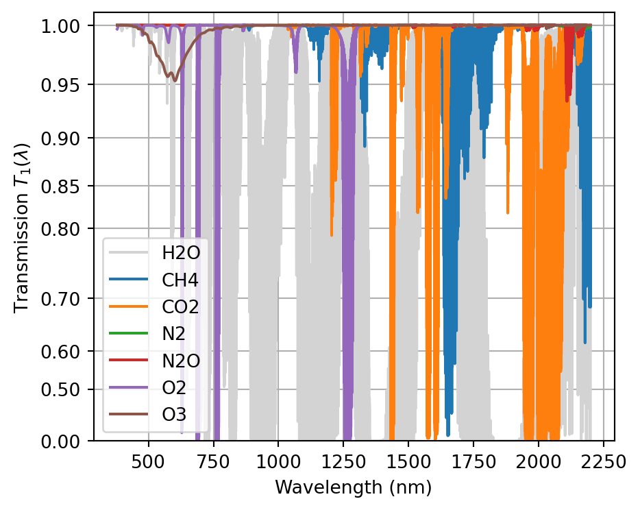
Gas optical depths per layer are obtained for each considered gas from the CKDMIP high-resolution line-by-line database (Hogan and Matricardi 2022) via the gatiab interface, where the atmospheric profiles are provided by AFGL (Anderson et al. 1986). By default the AFGL-US profile is used. These profiles are then integrated to obtain, for each gas, the total column optical depth at a high spectral resolution, \(T_1(\lambda)\), for unit air mass and a nominal gas quantity \(U = U_0\) (see Table 1).

Table 1: Nominal total column \(U_0\) for each atmospheric gas.

Gas	\(U_0\)
CH₄	9.46 × 10⁻⁴ g/cm²
CO₂	0.519 g/cm²
H₂O	1.42 g/cm²
N₂	782 g/cm²
N₂O	4.83 × 10⁻⁴ g/cm²
O₂	239 g/cm²
O₃	345 Dobson

The numerical values of \(T_1(\lambda)\) are stored in the file gaseous_absorption_model_gatiab_ckdmip_v1.nc for each gas.

Figure 1: High-resolution transmission \(T_1\) for all gases from 380 to 2200nm.

3.2 Integrated transmission model

3.2.1 Model description

The monochromatic transmission coefficient for an arbitrary air mass \(M\) and gas content \(U\) follows the Beer-Lambert law: and can be expressed as \(T_1(\lambda)^x\), where \(T_1(\lambda)\) is given for each gas at \(x=1\), with \(x = M \cdot U/U_0\) (air mass × gas content / nominal gas content). This expression is used for numerical reasons instead of the classical exponential law, so that \(T_1(\lambda) \in [0, 1]\).

For a given sensor band with SRF \(S(\lambda)\), the integrated transmission is defined as:

\[\bar{T}(x) = \frac{\int S(\lambda) T_1(\lambda)^x \, d\lambda}{\int S(\lambda) \, d\lambda} \tag{1}\]

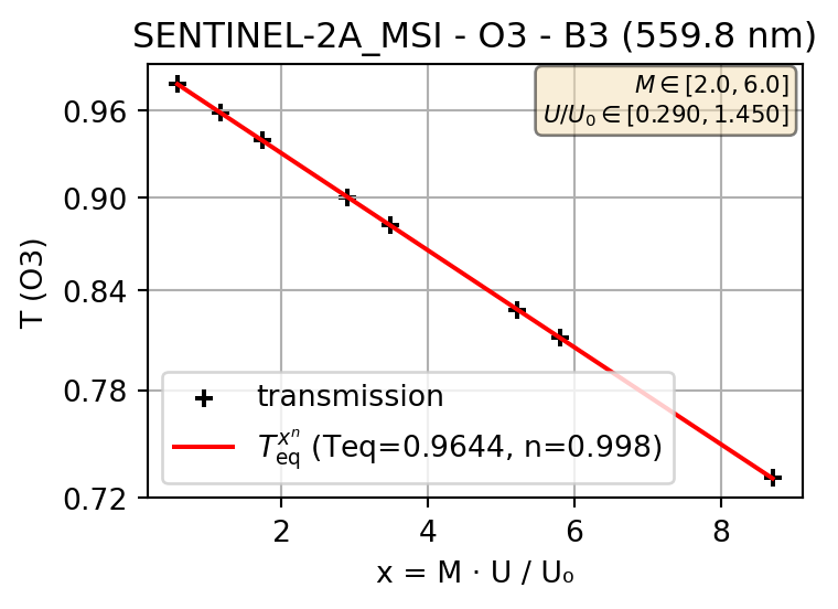
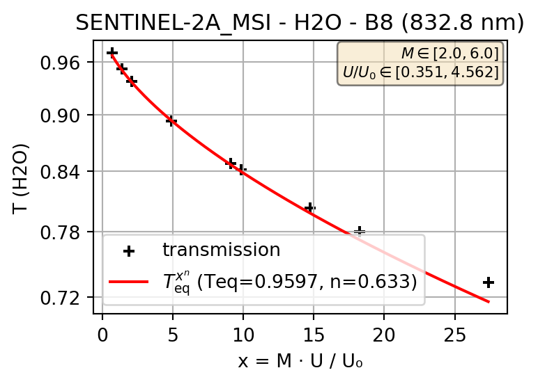
This integrated transmission does not necessarily follow the Beer-Lambert law, thus we propose a model in the form of \(\bar{T}(x) = T_\text{eq}^{x^n}\). On Figure 2 (a) the model closely follows the Beer-Lambert law (\(n \approx 1\)), but not on Figure 2 (b) (\(n=0.633\)).

The following plots illustrate the fitted transmission model \(\bar{T}(x) = T_\text{eq}^{x^n}\) for selected Sentinel-2A bands and gases.

(a) O₃, band B3 (559.8 nm).

(b) H₂O, band B8 (832.8 nm).

Figure 2: Transmission data for two combinations of MSI bands and gases, and the corresponding model \(T_\text{eq}^{(x^n)}\) (with numerical solving as detailed in next section). The ordinate axis is in log scale, thus n=1 corresponds to a straight line.

3.2.2 Numerical integration method

This section provides a method to calculate on the fly (the values of $T_eq$ and $n$ are not stored), for a given sensor band (SRF), the parameters of the model (\(T_\text{eq}\) and \(n\)). This method consists in calculating \(\bar{T}(x)\) and its derivative, for a single value of \(x = x_0\). This requires only two integrations of the SRF, and avoids integrating the SRF over many values of \(x\) for linear regression.

The derivative of the integrated transmission is:

\[\bar{T}'(x) = \frac{\int S(\lambda) T_1(\lambda)^x \ln T_1(\lambda) \, d\lambda}{\int S(\lambda) \, d\lambda} \tag{2}\]

We model the integrated transmission as:

\[\bar{T}(x) = T_\text{eq}^{(x^n)} \tag{3}\]

Then, the derivative of \(\bar{T}(x)\) at \(x=x_0\) is:

\[{\bar{T}'}(x_0) = n T_\text{eq}^{x_0^n} \ln T_\text{eq} \cdot x_0^{n-1}\]

Using \(\bar{T}(x_0) = T_\text{eq}^{x_0^n}\) and \(\ln \bar{T}(x_0) = x_0^n \ln T_\text{eq}\), this expression simplifies:

\[{\bar{T}'}(x_0) = n \cdot \frac{\bar{T}(x_0)\,\ln \bar{T}(x_0)}{x_0}\]

Then \(n\) can be solved by:

\[n = \frac{{\bar{T}'}(x_0) \cdot x_0}{\bar{T}(x_0) \cdot \ln \bar{T}(x_0)} \tag{4}\]

The values of \(\bar{T}(x_0)\) and \(\bar{T'}(x_0)\) are calculated using equations 1 and 2.

For \(T_\text{eq}\), and having solved for \(n\), Equation 3 gives:

\[T_\text{eq} = \bar{T}(x_0)^{\,x_0^{-n}} \tag{5}\]

In practice, this method is implemented in transmission_model_single with a default value of \(x_0 = 5\).

References

Anderson, G. P., S. A. Clough, F. X. Kneizys, J. H. Chetwynd, and E. P. Shettle. 1986. AFGL Atmospheric Constituent Profiles (0–120 Km). AFGL-TR-86-0110. Air Force Geophysics Laboratory.

Hogan, Robin J., and Marco Matricardi. 2022. “A Tool for Generating Fast k-Distribution Gas-Optics Models for Weather and Climate Applications.” Journal of Advances in Modeling Earth Systems 14 (10). https://doi.org/10.1029/2022ms003033.